Title 40
SECTION 1065.602
1065.602 Statistics.
§ 1065.602 Statistics.(a) Overview. This section contains equations and example calculations for statistics that are specified in this part. In this section we use the letter “y” to denote a generic measured quantity, the superscript over-bar “−“ to denote an arithmetic mean, and the subscript “ref” to denote the reference quantity being measured.
(b) Arithmetic mean. Calculate an arithmetic mean, y , as follows:
Example: N = 3 y1 = 10.60 y2 = 11.91 yN = y3 = 11.09 y = 11.20(c) Standard deviation. Calculate the standard deviation for a non-biased (e.g., N-1) sample, s, as follows:
Example: N = 3 y1 = 10.60 y2 = 11.91 yN = y3 = 11.09 y = 11.20 sy = 0.6619(d) Root mean square. Calculate a root mean square, rmsy, as follows:
Example: N = 3 y1 = 10.60 y2 = 11.91 yN = y3 = 11.09 rmsy = 11.21(e) Accuracy. Determine accuracy as described in this paragraph (e). Make multiple measurements of a standard quantity to create a set of observed values, yi, and compare each observed value to the known value of the standard quantity. The standard quantity may have a single known value, such as a gas standard, or a set of known values of negligible range, such as a known applied pressure produced by a calibration device during repeated applications. The known value of the standard quantity is represented by yrefi . If you use a standard quantity with a single value, yrefi would be constant. Calculate an accuracy value as follows:
Example: yref = 1800.0 N = 3 y1 = 1806.4 y2 = 1803.1 y3 = 1798.9 accuracy = 2.8(f) t-test. Determine if your data passes a t-test by using the following equations and tables:
(1) For an unpaired t-test, calculate the t statistic and its number of degrees of freedom, v, as follows:
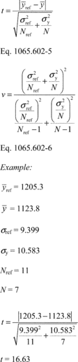
(2) For a paired t-test, calculate the t statistic and its number of degrees of freedom, v, as follows, noting that the εi are the errors (e.g., differences) between each pair of yrefi and yi:
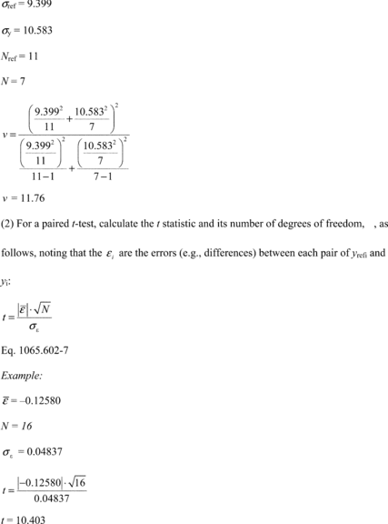
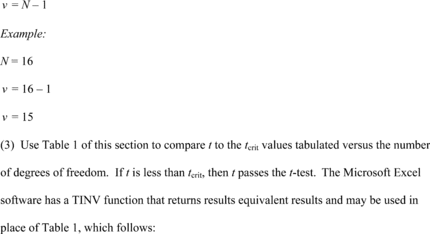
Table 1 of § 1065.602 - Critical t Values Versus Number of Degrees of Freedom, v 1
| n | Confidence | |
|---|---|---|
| 90% | 95% | |
| 1 | 6.314 | 12.706 |
| 2 | 2.920 | 4.303 |
| 3 | 2.353 | 3.182 |
| 4 | 2.132 | 2.776 |
| 5 | 2.015 | 2.571 |
| 6 | 1.943 | 2.447 |
| 7 | 1.895 | 2.365 |
| 8 | 1.860 | 2.306 |
| 9 | 1.833 | 2.262 |
| 10 | 1.812 | 2.228 |
| 11 | 1.796 | 2.201 |
| 12 | 1.782 | 2.179 |
| 13 | 1.771 | 2.160 |
| 14 | 1.761 | 2.145 |
| 15 | 1.753 | 2.131 |
| 16 | 1.746 | 2.120 |
| 18 | 1.734 | 2.101 |
| 20 | 1.725 | 2.086 |
| 22 | 1.717 | 2.074 |
| 24 | 1.711 | 2.064 |
| 26 | 1.706 | 2.056 |
| 28 | 1.701 | 2.048 |
| 30 | 1.697 | 2.042 |
| 35 | 1.690 | 2.030 |
| 40 | 1.684 | 2.021 |
| 50 | 1.676 | 2.009 |
| 70 | 1.667 | 1.994 |
| 100 | 1.660 | 1.984 |
| 1000 + | 1.645 | 1.960 |
1 Use linear interpolation to establish values not shown here.
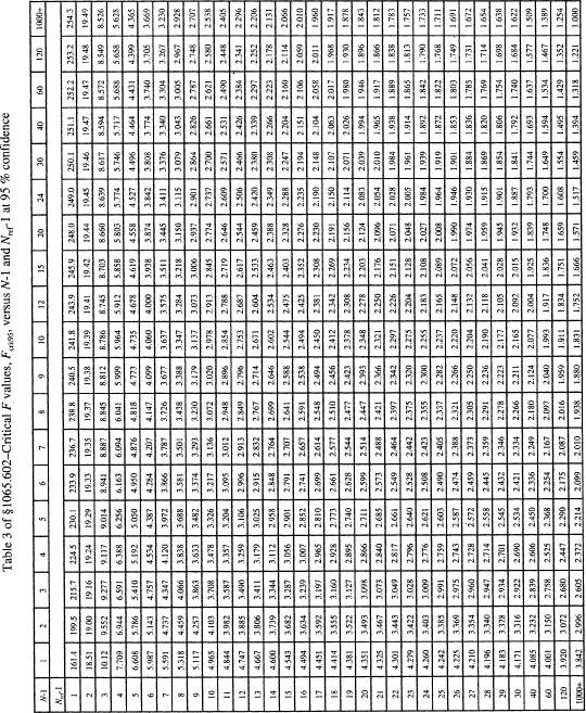
(g) F-test. Calculate the F statistic as follows:
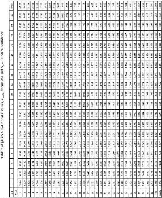
Example: F = 1.268(1) For a 90% confidence F-test, use Table 2 of this section to compare F to the Fcrit90 values tabulated versus (N−1) and (Nref−1). If F is less than Fcrit90, then F passes the F-test at 90% confidence.
(2) For a 95% confidence F-test, use Table 3 of this section to compare F to the Fcrit95 values tabulated versus (N−1) and (Nref−1). If F is less than Fcrit95, then F passes the F-test at 95% confidence.
(h) Slope. Calculate a least-squares regression slope, a1y, as follows:
 Example:
N = 6000 y1 = 2045.8 y = 1050.1 yref 1
= 2045.0 y ref = 1055.3
Example:
N = 6000 y1 = 2045.8 y = 1050.1 yref 1
= 2045.0 y ref = 1055.3  a1y =
1.0110
a1y =
1.0110
(i) Intercept. Calculate a least-squares regression intercept, a0y, as follows:
Example: y = 1050.1 a1y = 1.0110 y ref = 1055.3 a0y = 1050.1 − (1.0110 · 1055.3) a0y = −16.8083(j) Standard estimate of error. Calculate a standard estimate of error, SEE, as follows:
 Eq.
1065.602-11 Example: N = 6000 y1 = 2045.8 a0y
= -16.8083 a1y = 1.0110 yref1 = 2045.0
Eq.
1065.602-11 Example: N = 6000 y1 = 2045.8 a0y
= -16.8083 a1y = 1.0110 yref1 = 2045.0  SEEy =
5.348
SEEy =
5.348
(k) Coefficient of determination. Calculate a coefficient of determination, r 2, as follows:
Example: N = 6000 y1 = 2045.8 a0y = −16.8083 a1y = 1.0110 yrefi = 2045.0 y = 1480.5(l) Flow-weighted mean concentration. In some sections of this part, you may need to calculate a flow-weighted mean concentration to determine the applicability of certain provisions. A flow-weighted mean is the mean of a quantity after it is weighted proportional to a corresponding flow rate. For example, if a gas concentration is measured continuously from the raw exhaust of an engine, its flow-weighted mean concentration is the sum of the products of each recorded concentration times its respective exhaust molar flow rate, divided by the sum of the recorded flow rate values. As another example, the bag concentration from a CVS system is the same as the flow-weighted mean concentration because the CVS system itself flow-weights the bag concentration. You might already expect a certain flow-weighted mean concentration of an emission at its standard based on previous testing with similar engines or testing with similar equipment and instruments. If you need to estimate your expected flow-weighted mean concentration of an emission at its standard, we recommend using the following examples as a guide for how to estimate the flow-weighted mean concentration expected at the standard. Note that these examples are not exact and that they contain assumptions that are not always valid. Use good engineering judgment to determine if you can use similar assumptions.
(1) To estimate the flow-weighted mean raw exhaust NOX concentration from a turbocharged heavy-duty compression-ignition engine at a NOX standard of 2.5 g/(kW · hr), you may do the following:
(i) Based on your engine design, approximate a map of maximum torque versus speed and use it with the applicable normalized duty cycle in the standard-setting part to generate a reference duty cycle as described in § 1065.610. Calculate the total reference work, Wref, as described in § 1065.650. Divide the reference work by the duty cycle's time interval, Δtdutycycle, to determine mean reference power, Pref.
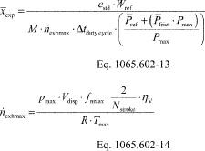
(ii) Based on your engine design, estimate maximum power, Pmax, the design speed at maximum power, fnmax, the design maximum intake manifold boost pressure, pinmax, and temperature, Tinmax. Also, estimate a mean fraction of power that is lost due to friction and pumping, p frict. Use this information along with the engine displacement volume, Vdisp, an approximate volumetric efficiency, hV, and the number of engine strokes per power stroke (two-stroke or four-stroke), Nstroke, to estimate the maximum raw exhaust molar flow rate, n exhmax.
(iii) Use your estimated values as described in the following example calculation:
 Example:
eNOx = 2.5 g/(kW · hr) Wref = 11.883 kW · hr
MNOx = 46.0055 g/mol = 46.0055 · 10−6 g/µmol
Δtdutycycle = 20 min = 1200 s P ref = 35.65 kW
P frict = 15% Pmax = 125 kW pmax = 300 kPa =
300,000 Pa Vdisp = 3.0 l = 0.0030 m 3/r fnmax = 2,800
r/min = 46.67 r/s Nstroke = 4 ηV = 0.9 R = 8.314472
J/(mol · K) Tmax = 348.15 K
Example:
eNOx = 2.5 g/(kW · hr) Wref = 11.883 kW · hr
MNOx = 46.0055 g/mol = 46.0055 · 10−6 g/µmol
Δtdutycycle = 20 min = 1200 s P ref = 35.65 kW
P frict = 15% Pmax = 125 kW pmax = 300 kPa =
300,000 Pa Vdisp = 3.0 l = 0.0030 m 3/r fnmax = 2,800
r/min = 46.67 r/s Nstroke = 4 ηV = 0.9 R = 8.314472
J/(mol · K) Tmax = 348.15 K 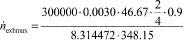 n exhmax =
6.53 mol/s
n exhmax =
6.53 mol/s 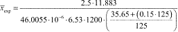 x exp =
189.4 µmol/mol
x exp =
189.4 µmol/mol
(2) To estimate the flow-weighted mean NMHC concentration in a CVS from a naturally aspirated nonroad spark-ignition engine at an NMHC standard of 0.5 g/(kW · hr), you may do the following:
(i) Based on your engine design, approximate a map of maximum torque versus speed and use it with the applicable normalized duty cycle in the standard-setting part to generate a reference duty cycle as described in § 1065.610. Calculate the total reference work, Wref, as described in § 1065.650.
(ii) Multiply your CVS total molar flow rate by the time interval of the duty cycle, Δtdutycycle. The result is the total diluted exhaust flow of the ndexh.
(iii) Use your estimated values as described in the following example calculation:
Example: eNMHC = 1.5 g/(kW · hr) Wref = 5.389 kW · hr MNMHC = 13.875389 g/mol = 13.875389 · 10−6 g/µmol n dexh = 6.021 mol/s Δtdutycycle = 30 min = 1800 s x NMHC = 53.8 µmol/mol [70 FR 40516, July 13, 2005, as amended at 73 FR 37324, June 30, 2008; 75 FR 23044, Apr. 30, 2010; 76 FR 57452, Sept. 15, 2011; 79 FR 23779, Apr. 28, 2014; 81 FR 74170, Oct. 25, 2016]