Title 40
SECTION 1066.625
1066.625 Flow meter calibration calculations.
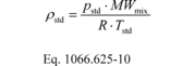
§ 1066.625 Flow meter calibration calculations.This section describes the calculations for calibrating various flow meters based on mass flow rates. Calibrate your flow meter according to 40 CFR 1065.640 instead if you calculate emissions based on molar flow rates.
(a) PDP calibration. Perform the following steps to calibrate a PDP flow meter:
(1) Calculate PDP volume pumped per revolution, Vrev, for each restrictor position from the mean values determined in § 1066.140:
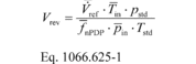 Where:
V ref = mean flow rate of the reference flow meter. Tin =
mean temperature at the PDP inlet. pstd = standard pressure
= 101.325 kPa. f nPDP = mean PDP speed. Pin = mean static
absolute pressure at the PDP inlet. Tstd = standard
temperature = 293.15 K. Example: V ref = 0.1651 m 3/s Tin =
299.5 K pstd = 101.325 kPa f nPDP = 1205.1 r/min =
20.085 r/s Pin = 98.290 kPa Tstd = 293.15 K
Where:
V ref = mean flow rate of the reference flow meter. Tin =
mean temperature at the PDP inlet. pstd = standard pressure
= 101.325 kPa. f nPDP = mean PDP speed. Pin = mean static
absolute pressure at the PDP inlet. Tstd = standard
temperature = 293.15 K. Example: V ref = 0.1651 m 3/s Tin =
299.5 K pstd = 101.325 kPa f nPDP = 1205.1 r/min =
20.085 r/s Pin = 98.290 kPa Tstd = 293.15 K 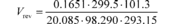 Vrev =
0.00866 m 3/r
Vrev =
0.00866 m 3/r
(2) Calculate a PDP slip correction factor, Ks for each restrictor position from the mean values determined in § 1066.140:
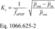 Where:
f mPDP = mean PDP speed. p out = mean static absolute
pressure at the PDP outlet. p in = mean static absolute
pressure at the PDP inlet.
Where:
f mPDP = mean PDP speed. p out = mean static absolute
pressure at the PDP outlet. p in = mean static absolute
pressure at the PDP inlet. 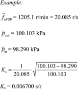
(3) Perform a least-squares regression of Vrev, versus Ks, by calculating slope, a1, and intercept, a0, as described in 40 CFR 1065.602.
(4) Repeat the procedure in paragraphs (a)(1) through (3) of this section for every speed that you run your PDP.
(5) The following example illustrates a range of typical values for different PDP speeds:
Table 1 of § 1066.625 - Example of PDP Calibration Data
| f nPDP (revolution/s) |
a1 (m 3/s) |
a0 (m 3/revolution) |
|---|---|---|
| 12.6 | 0.841 | 0.056 |
| 16.5 | 0.831 | −0.013 |
| 20.9 | 0.809 | 0.028 |
| 23.4 | 0.788 | −0.061 |
(6) For each speed at which you operate the PDP, use the appropriate regression equation from this paragraph (a) to calculate flow rate during emission testing as described in § 1066.630.
(b) SSV calibration. The equations governing SSV flow assume one-dimensional isentropic inviscid flow of an ideal gas. Paragraph (b)(2)(iv) of this section describes other assumptions that may apply. If good engineering judgment dictates that you account for gas compressibility, you may either use an appropriate equation of state to determine values of Z as a function of measured pressure and temperature, or you may develop your own calibration equations based on good engineering judgment. Note that the equation for the flow coefficient, Cf, is based on the ideal gas assumption that the isentropic exponent, g, is equal to the ratio of specific heats, Cp/Cv. If good engineering judgment dictates using a real gas isentropic exponent, you may either use an appropriate equation of state to determine values of γ as a function of measured pressure and temperature, or you may develop your own calibration equations based on good engineering judgment.
(1) Calculate volume flow rate at standard reference conditions, V std, as follows
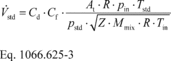 Where:
Cd = discharge coefficient, as determined in paragraph
(b)(2)(i) of this section. Cf = flow coefficient, as
determined in paragraph (b)(2)(ii) of this section. At =
cross-sectional area at the venturi throat. R = molar gas
constant. pin = static absolute pressure at the venturi
inlet. Tstd = standard temperature. pstd = standard
pressure. Z = compressibility factor. Mmix = molar
mass of gas mixture. Tin = absolute temperature at the
venturi inlet.
Where:
Cd = discharge coefficient, as determined in paragraph
(b)(2)(i) of this section. Cf = flow coefficient, as
determined in paragraph (b)(2)(ii) of this section. At =
cross-sectional area at the venturi throat. R = molar gas
constant. pin = static absolute pressure at the venturi
inlet. Tstd = standard temperature. pstd = standard
pressure. Z = compressibility factor. Mmix = molar
mass of gas mixture. Tin = absolute temperature at the
venturi inlet.
(2) Perform the following steps to calibrate an SSV flow meter:
(i) Using the data collected in § 1066.140, calculate Cd for each flow rate using the following equation:
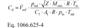 Where:
V ref = measured volume flow rate from the reference flow
meter.
Where:
V ref = measured volume flow rate from the reference flow
meter.
(ii) Use the following equation to calculate Cf for each flow rate:
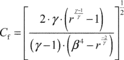 Where: g
= isentropic exponent. For an ideal gas, this is the ratio of
specific heats of the gas mixture, Cp/Cv. r =
pressure ratio, as determined in paragraph (b)(2)(iii) of this
section. b = ratio of venturi throat diameter to inlet diameter.
Where: g
= isentropic exponent. For an ideal gas, this is the ratio of
specific heats of the gas mixture, Cp/Cv. r =
pressure ratio, as determined in paragraph (b)(2)(iii) of this
section. b = ratio of venturi throat diameter to inlet diameter.
(iii) Calculate r using the following equation:
 Where:
Δp = differential static pressure, calculated as venturi
inlet pressure minus venturi throat pressure.
Where:
Δp = differential static pressure, calculated as venturi
inlet pressure minus venturi throat pressure.
(iv) You may apply any of the following simplifying assumptions or develop other values as appropriate for your test configuration, consistent with good engineering judgment:
(A) For raw exhaust, diluted exhaust, and dilution air, you may assume that the gas mixture behaves as an ideal gas (Z = 1).
(B) For raw exhaust, you may assume g = 1.385.
(C) For diluted exhaust and dilution air, you may assume g = 1.399.
(D) For diluted exhaust and dilution air, you may assume the molar mass of the mixture, Mmix, is a function only of the amount of water in the dilution air or calibration air, as follows:
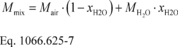 Where:
Mair = molar mass of dry air.xH2O = amount of H2O in
the dilution air or calibration air, determined as described in 40
CFR 1065.645. MH2O = molar mass of water. Example:
Mair = 28.96559 g/mol xH2O = 0.0169 mol/mol
MH2O = 18.01528 g/mol Mmix = 28.96559 · (1 − 0.0169)
+ 18.01528 · 0.0169 Mmix = 28.7805 g/mol
Where:
Mair = molar mass of dry air.xH2O = amount of H2O in
the dilution air or calibration air, determined as described in 40
CFR 1065.645. MH2O = molar mass of water. Example:
Mair = 28.96559 g/mol xH2O = 0.0169 mol/mol
MH2O = 18.01528 g/mol Mmix = 28.96559 · (1 − 0.0169)
+ 18.01528 · 0.0169 Mmix = 28.7805 g/mol
(E) For diluted exhaust and dilution air, you may assume a constant molar mass of the mixture, Mmix, for all calibration and all testing if you control the amount of water in dilution air and in calibration air, as illustrated in the following table:
Table 2 of § 1066.625 - Examples of Dilution Air and Calibration Air Dewpoints at Which You May Assume a Constant Mmix
| If calibration Tdew ( °C) is . . . | assume the following constant Mmix (g/mol) . . . |
for the following ranges of Tdew ( °C) during emission tests a |
|---|---|---|
| ≤0 | 28.96559 | ≤18 |
| 0 | 28.89263 | ≤21 |
| 5 | 28.86148 | ≤22 |
| 10 | 28.81911 | ≤24 |
| 15 | 28.76224 | ≤26 |
| 20 | 28.68685 | −8 to 28 |
| 25 | 28.58806 | 12 to 31 |
| 30 | 28.46005 | 23 to 34 |
a The specified ranges are valid for all calibration and emission testing over the atmospheric pressure range (80.000 to 103.325) kPa.
(v) The following example illustrates the use of the governing equations to calculate Cd of an SSV flow meter at one reference flow meter value:
V ref = 2.395 m 3/s Z = 1 Mmix = 28.7805 g/mol = 0.0287805 kg/mol R = 8.314472 J/(mol·K) = 8.314472 (m 2·kg)/(s 2·mol·K) Tin = 298.15 K At = 0.01824 m 2 pin = 99.132 kPa = 99132 Pa = 99132 kg/(m·s 2) g = 1.399 b = 0.8 Δp = 7.653 kPa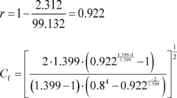 Cf = 0.472
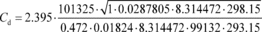 Cd
= 0.985
Cd
= 0.985
(vi) Calculate the Reynolds number, Re#, for each reference flow rate at standard conditions, V refstd, using the throat diameter of the venturi, dt, and the air density at standard conditions, rstd. Because the dynamic viscosity, m, is needed to compute Re#, you may use your own fluid viscosity model to determine m for your calibration gas (usually air), using good engineering judgment. Alternatively, you may use the Sutherland three-coefficient viscosity model to approximate m, as shown in the following sample calculation for Re#:
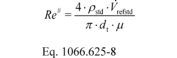
Where, using the Sutherland three-coefficient viscosity model:
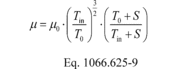 Where: m0
= Sutherland reference viscosity. T0 = Sutherland reference
temperature. S = Sutherland constant.
Where: m0
= Sutherland reference viscosity. T0 = Sutherland reference
temperature. S = Sutherland constant.
Table 3 of § 1066.625 - Sutherland Three-Coefficient Viscosity Model Parameters
| Gas 1 | m0 | T0 | S | Temperature range within ±2% error 2 | Pressure limit 2 |
|---|---|---|---|---|---|
| kg/(m·s) | K | K | K | kPa | |
| Air | 1.716·10−5 | 273 | 111 | 170 to 1900 | ≤1800. |
| CO2 | 1.370·10−5 | 273 | 222 | 190 to 1700 | ≤3600. |
| H2O | 1.12·10−5 | 350 | 1064 | 360 to 1500 | ≤10000. |
| O2 | 1.919·10−5 | 273 | 139 | 190 to 2000 | ≤2500. |
| N2 | 1.663·10−5 | 273 | 107 | 100 to 1500 | ≤1600. |
1 Use tabulated parameters only for the pure gases, as listed. Do not combine parameters in calculations to calculate viscosities of gas mixtures.
2 The model results are valid only for ambient conditions in the specified ranges.
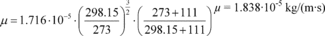 Tin = 298.15 K dt = 152.4 mm = 0.1524 m rstd = 1.1509
kg/m 3
Tin = 298.15 K dt = 152.4 mm = 0.1524 m rstd = 1.1509
kg/m 3 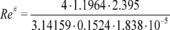 Re# = 1.3027·10 6
(vii) Calculate r using the following equation:
 Example:
 ρstd = 1.1964 kg/m 3
(viii) Create an equation for Cd as a function of Re#, using paired values of the two quantities. The equation may involve any mathematical expression, including a polynomial or a power series. The following equation is an example of a commonly used mathematical expression for relating Cd and Re#:

(ix) Perform a least-squares regression analysis to determine the best-fit coefficients for the equation and calculate SEE as described in 40 CFR 1065.602.
(x) If the equation meets the criterion of SEE ≤0.5% ⋅ Cdmax, you may use the equation for the corresponding range of Re#, as described in § 1066.630(b).
(xi) If the equation does not meet the specified statistical criteria, you may use good engineering judgment to omit calibration data points; however, you must use at least seven calibration data points to demonstrate that you meet the criterion. For example, this may involve narrowing the range of flow rates for a better curve fit.
(xii) Take corrective action if the equation does not meet the specified statistical criterion even after omitting calibration data points. For example, select another mathematical expression for the Cd versus Re# equation, check for leaks, or repeat the calibration process. If you must repeat the calibration process, we recommend applying tighter tolerances to measurements and allowing more time for flows to stabilize.
(xiii) Once you have an equation that meets the specified statistical criterion, you may use the equation only for the corresponding range of Re#.
(c) CFV calibration. Some CFV flow meters consist of a single venturi and some consist of multiple venturis where different combinations of venturis are used to meter different flow rates. For CFV flow meters that consist of multiple venturis, either calibrate each venturi independently to determine a separate calibration coefficient, Kv, for each venturi, or calibrate each combination of venturis as one venturi by determining Kv for the system.
(1) To determine Kv for a single venturi or a combination of venturis, perform the following steps:
(i) Calculate an individual Kv for each calibration set point for each restrictor position using the following equation:
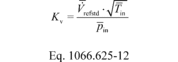 Where:
V refstd= mean flow rate from the reference flow meter,
corrected to standard reference conditions. T in= mean
temperature at the venturi inlet. P in= mean static absolute
pressure at the venturi inlet.
Where:
V refstd= mean flow rate from the reference flow meter,
corrected to standard reference conditions. T in= mean
temperature at the venturi inlet. P in= mean static absolute
pressure at the venturi inlet.
(ii) Calculate the mean and standard deviation of all the Kv values (see 40 CFR 1065.602). Verify choked flow by plotting Kv as a function of pin. Kv will have a relatively constant value for choked flow; as vacuum pressure increases, the venturi will become unchoked and Kv will decrease. Paragraphs (c)(1)(iii) through (viii) of this section describe how to verify your range of choked flow.
(iii) If the standard deviation of all the Kv values is less than or equal to 0.3% of the mean Kv, use the mean Kv in Eq. 1066.630-7, and use the CFV only up to the highest venturi pressure ratio, r, measured during calibration using the following equation:
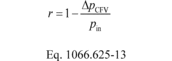 Where:
ΔpCFV = differential static pressure; venturi inlet minus
venturi outlet. pin = mean static absolute pressure at the
venturi inlet.
Where:
ΔpCFV = differential static pressure; venturi inlet minus
venturi outlet. pin = mean static absolute pressure at the
venturi inlet.
(iv) If the standard deviation of all the Kv values exceeds 0.3% of the mean Kv, omit the Kv value corresponding to the data point collected at the highest r measured during calibration.
(v) If the number of remaining data points is less than seven, take corrective action by checking your calibration data or repeating the calibration process. If you repeat the calibration process, we recommend checking for leaks, applying tighter tolerances to measurements and allowing more time for flows to stabilize.
(vi) If the number of remaining Kv values is seven or greater, recalculate the mean and standard deviation of the remaining Kv values.
(vii) If the standard deviation of the remaining Kv values is less than or equal to 0.3% of the mean of the remaining Kv, use that mean Kv in Eq 1066.630-7, and use the CFV values only up to the highest r associated with the remaining Kv.
(viii) If the standard deviation of the remaining Kv still exceeds 0.3% of the mean of the remaining Kv values, repeat the steps in paragraph (c)(1)(iv) through (vii) of this section.
(2) During exhaust emission tests, monitor sonic flow in the CFV by monitoring r. Based on the calibration data selected to meet the standard deviation criterion in paragraphs (c)(1)(iv) and (vii) of this section, in which Kv is constant, select the data values associated with the calibration point with the lowest absolute venturi inlet pressure to determine the r limit. Calculate r during the exhaust emission test using Eq. 1066.625-8 to demonstrate that the value of r during all emission tests is less than or equal to the r limit derived from the CFV calibration data.
[79 FR 23823, Apr. 28, 2016, as amended at 81 FR 74208, Oct. 25, 2016]